Note
Go to the end to download the full example code. or to run this example in your browser via Binder
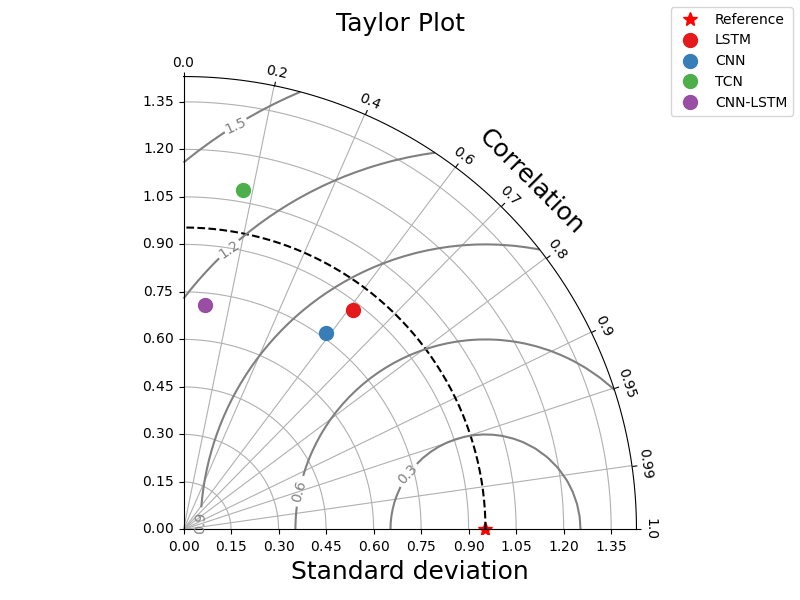
o. taylor plot
This file shows the usage of taylor_plot() function.
A Taylor plot can be used to show statistical summary of one or more measurements/models.
import numpy as np
from easy_mpl import taylor_plot
from easy_mpl.utils import version_info

version_info()

# sphinx_gallery_thumbnail_number = -1
{'easy_mpl': '0.21.5', 'matplotlib': '3.9.4', 'numpy': '2.0.2', 'pandas': '2.2.3', 'scipy': '1.13.1'}
# The desired covariance matrix.
cov = np.array(
       [[1,  0.8, 0.6, 0.4, 0.2],
       [0.8, 1.2, 0.8, 0.6, 0.4],
       [0.6, 0.8, 0.8, 0.8, 0.6],
       [0.4, 0.6, 0.8, 1.4, 0.8],
       [0.2, 0.4, 0.6, 0.8, 0.6]]
)

# Generate the random samples.
rng = np.random.default_rng(313)
data = rng.multivariate_normal(np.zeros(5), cov, size=100)
print(data.shape)

observations =  data[:, 0]
simulations =  {"LSTM": data[:, 1],
            "CNN": data[:, 2],
            "TCN": data[:, 3],
            "CNN-LSTM": data[:, 4]}
_ = taylor_plot(observations=observations,
            simulations=simulations,
            title="Taylor Plot")
/home/docs/checkouts/readthedocs.org/user_builds/easy-mpl/checkouts/latest/examples/taylor_plot.py:35: RuntimeWarning: covariance is not symmetric positive-semidefinite.
  data = rng.multivariate_normal(np.zeros(5), cov, size=100)
(100, 5)
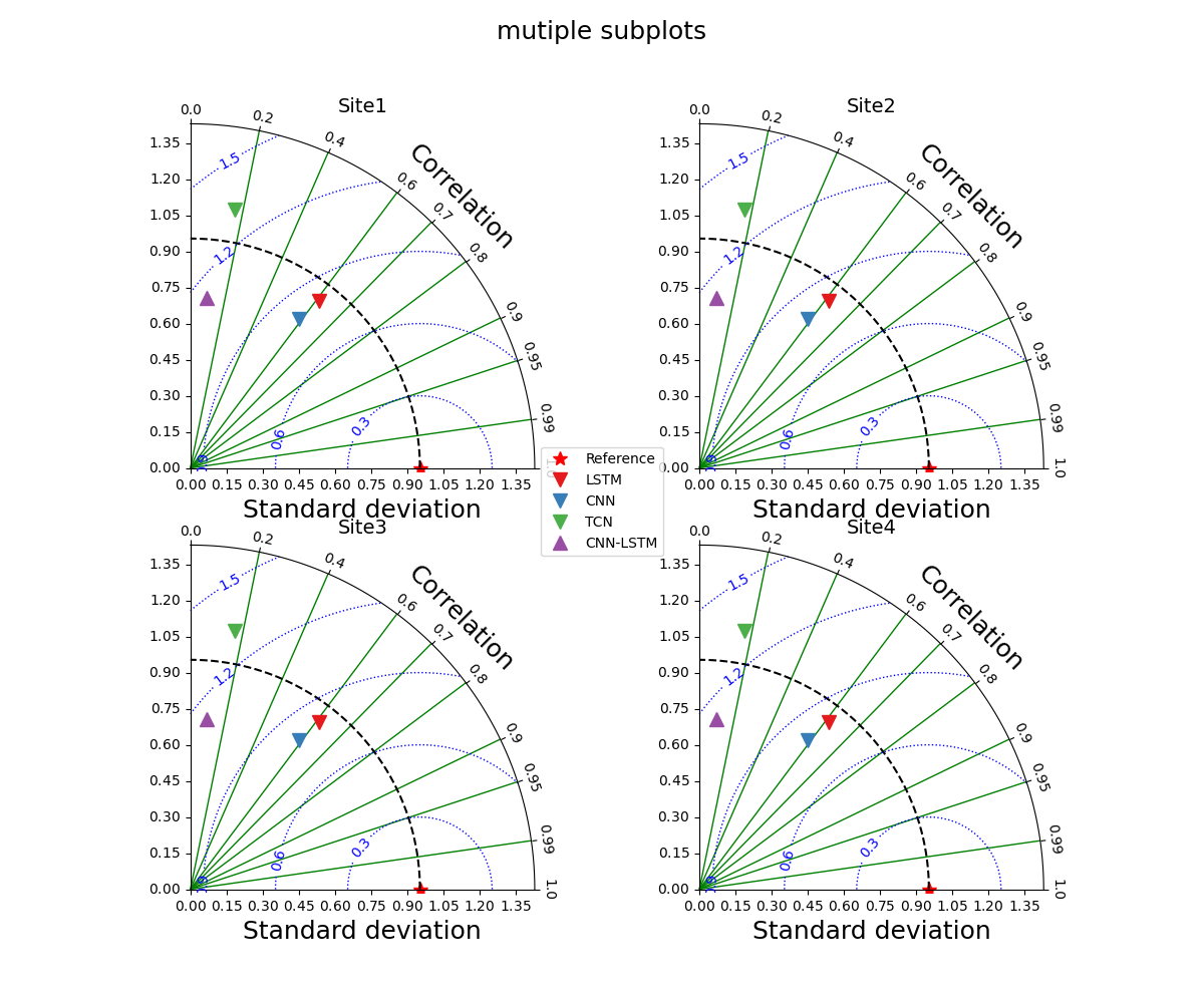
multiple taylor plots in one figure
def create_data(cov, seed=313, mu=np.zeros(5), size=100):

    # Generate the random samples.
    rng = np.random.default_rng(seed)

    return rng.multivariate_normal(np.zeros(5), cov, size=size)

cov1 = np.array(
    [[1,  0.8, 0.6, 0.4, 0.2],
    [0.8, 1.2, 0.8, 0.6, 0.4],
    [0.6, 0.8, 0.8, 0.8, 0.6],
    [0.4, 0.6, 0.8, 1.4, 0.8],
    [0.2, 0.4, 0.6, 0.8, 0.6]]
)

cov2 = np.array(
    [[1,  0.8, 0.6, 0.4, 0.2],
    [0.8, 1.2, 0.8, 0.6, 0.4],
    [0.6, 0.8, 0.8, 0.8, 0.6],
    [0.4, 0.6, 0.8, 1.4, 0.8],
    [0.2, 0.4, 0.6, 0.8, 0.6]]
)

cov3 = np.array(
    [[1,  0.8, 0.6, 0.4, 0.2],
    [0.8, 1.2, 0.8, 0.6, 0.4],
    [0.6, 0.8, 0.8, 0.8, 0.6],
    [0.4, 0.6, 0.8, 1.4, 0.8],
    [0.2, 0.4, 0.6, 0.8, 0.6]]
)

cov4 = np.array(
    [[1,  0.8, 0.6, 0.4, 0.2],
    [0.8, 1.2, 0.8, 0.6, 0.4],
    [0.6, 0.8, 0.8, 0.8, 0.6],
    [0.4, 0.6, 0.8, 1.4, 0.8],
    [0.2, 0.4, 0.6, 0.8, 0.6]]
)

site1_data = create_data(cov1)
site2_data = create_data(cov2)
site3_data = create_data(cov3)
site4_data = create_data(cov4)

observations = {
    'site1': site1_data[:, 0],
    'site2': site2_data[:, 0],
    'site3': site3_data[:, 0],
    'site4': site4_data[:, 0],
}

simulations = {
    "site1": {"LSTM": site1_data[:, 1],
                "CNN": site1_data[:, 2],
                "TCN": site1_data[:, 3],
                "CNN-LSTM": site1_data[:, 4]},

    "site2": {"LSTM": site2_data[:, 1],
                "CNN": site2_data[:, 2],
                "TCN": site2_data[:, 3],
                "CNN-LSTM": site2_data[:, 4]},

    "site3": {"LSTM": site3_data[:, 1],
                "CNN": site3_data[:, 2],
                "TCN": site3_data[:, 3],
                "CNN-LSTM": site3_data[:, 4]},

    "site4": {"LSTM": site4_data[:, 1],
                "CNN": site4_data[:, 2],
                "TCN": site4_data[:, 3],
                "CNN-LSTM": site4_data[:, 4]},
}

# define positions of subplots

rects = dict(site1=221, site2=222, site3=223, site4=224)

_ = taylor_plot(observations=observations,
            simulations=simulations,
            axis_locs=rects,
            plot_bias=True,
            cont_kws={'colors': 'blue', 'linewidths': 1.0, 'linestyles': 'dotted'},
            grid_kws={'axis': 'x', 'color': 'g', 'lw': 1.0},
            title="mutiple subplots")
/home/docs/checkouts/readthedocs.org/user_builds/easy-mpl/checkouts/latest/examples/taylor_plot.py:55: RuntimeWarning: covariance is not symmetric positive-semidefinite.
  return rng.multivariate_normal(np.zeros(5), cov, size=size)
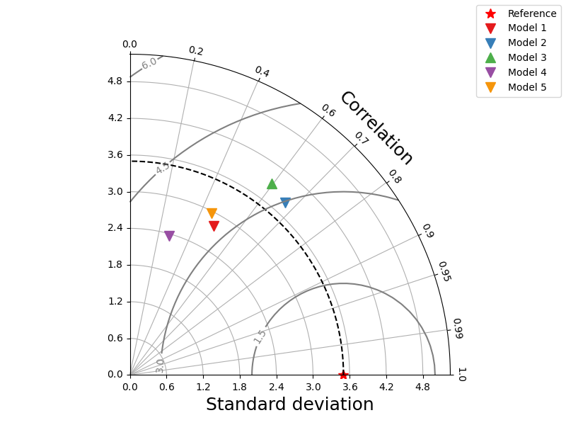
using statistics instead of arrays
observations = {'std': 3.5}
predictions = {   # pbias is optional
        'Model 1': {'std': 2.80068, 'corr_coeff': 0.49172, 'pbias': -8.85},
        'Model 2': {'std': 3.8, 'corr_coeff': 0.67, 'pbias': -19.76},
        'Model 3': {'std': 3.9, 'corr_coeff': 0.596, 'pbias': 7.81},
        'Model 4': {'std': 2.36, 'corr_coeff': 0.27, 'pbias': -22.78},
        'Model 5': {'std': 2.97, 'corr_coeff': 0.452, 'pbias': -7.99}}


_ = taylor_plot(observations,
    predictions)
with customized markers
cov = np.array(
    [[1, 0.8, 0.6, 0.4, 0.2],
     [0.8, 1.2, 0.8, 0.6, 0.4],
     [0.6, 0.8, 0.8, 0.8, 0.6],
     [0.4, 0.6, 0.8, 1.4, 0.8],
     [0.2, 0.4, 0.6, 0.8, 0.6]]
)

data = create_data(cov)

observations = data[:, 0]
simulations = {"LSTM": data[:, 1],
               "CNN": data[:, 2],
               "TCN": data[:, 3],
               "CNN-LSTM": data[:, 4]}
_ = taylor_plot(observations=observations,
                simulations=simulations,
                marker_kws={'markersize': 10, 'markeredgewidth': 1.5,
                            'markeredgecolor': 'black', 'lw': 0.0})

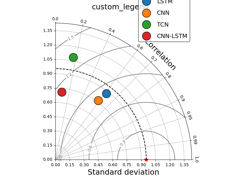
with customizing bbox
_ = taylor_plot(observations=observations,
            simulations=simulations,
            title="custom_legend",
            leg_kws={'facecolor': 'white',
                'edgecolor': 'black','bbox_to_anchor':(0.80, 1.1),
                'fontsize': 14, 'labelspacing': 1.0},
                marker_kws = {'ms':'20', 'markeredgecolor': 'k', 'lw': 0.0},
                )
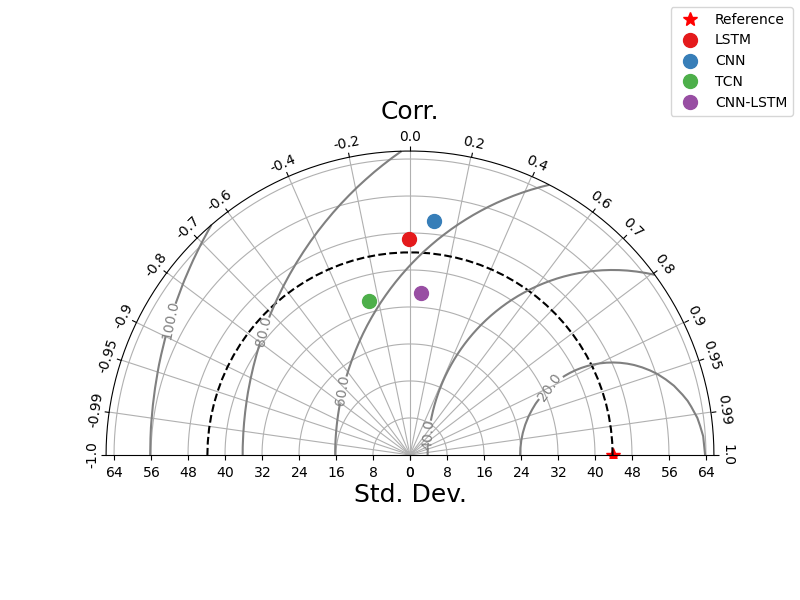
using extended horizontal axis to show the points which have negative correlation.
we can also change axis labels
np.random.seed(313)
observations = np.random.normal(20, 40, 10)
simus = {"LSTM": np.random.normal(20, 40, 10),
         "CNN": np.random.normal(20, 40, 10),
         "TCN": np.random.normal(20, 40, 10),
         "CNN-LSTM": np.random.normal(20, 40, 10)}
taylor_plot(observations=observations,
            simulations=simus,
            extend=True,
            corr_alias='Corr.',
            std_alias='Std. Dev.')
<Figure size 800x600 with 1 Axes>
Total running time of the script: (0 minutes 2.334 seconds)