c. imshow

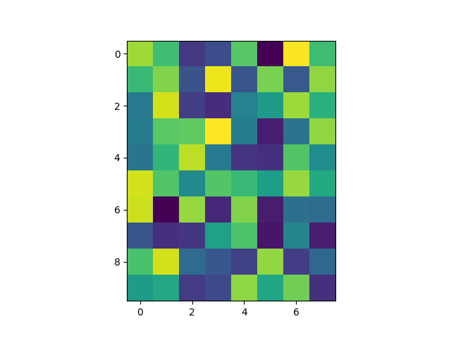
This file shows the usage of imshow() function.

imshow can be used to draw heatmap of a two-dimensional array/data.

# sphinx_gallery_thumbnail_number = 3

import numpy as np
import pandas as pd
import matplotlib.pyplot as plt

from easy_mpl import imshow
from easy_mpl.utils import version_info, despine_axes

version_info()  # print version information of all the packages being used

{'easy_mpl': '0.21.5', 'matplotlib': '3.9.4', 'numpy': '2.0.2', 'pandas': '2.2.3', 'scipy': '1.13.1'}

x = np.random.random((10, 8))

_ = imshow(x)

_ = imshow(x, annotate=True)

show colorbar

_ = imshow(x, colorbar=True)

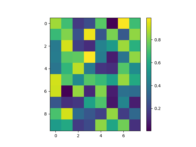
do not show border around colorbar

_ = imshow(x, colorbar=True, cbar_params={"border": False})

Move the colorbar below the heatmap

_ = imshow(x, colorbar=True, cbar_params={"border": False, 'pad': 0.4,
                                          "orientation":"horizontal"})

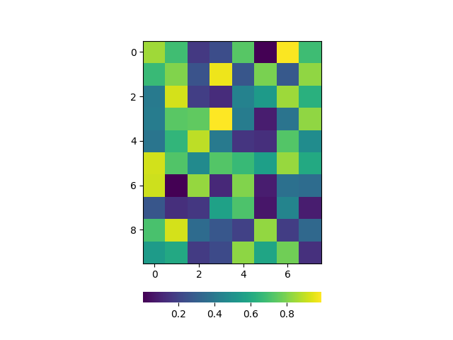
show white grid line

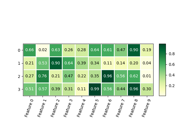
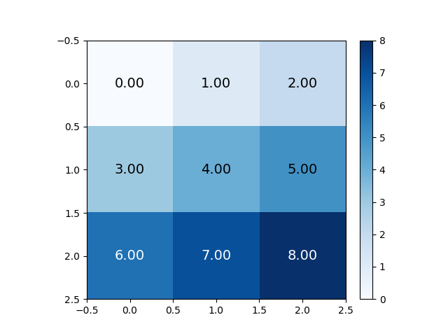
data = np.random.random((4, 10))

_ = imshow(data, cmap="YlGn",
       xticklabels=[f"Feature {i}" for i in range(data.shape[1])],
       grid_params={'border': True, 'color': 'w', 'linewidth': 2},
           annotate=True,
       colorbar=True)

we can specify color of text in each box of imshow for annotation For this, textcolors must a numpy array of shape same as that of data. Each value in this numpy array will define color for corresponding box annotation.

data = np.arange(9).reshape((3,3))

_ = imshow(data, cmap="Blues",
       annotate=True,
       annotate_kws={
              "textcolors": np.array([['black', 'black', 'black'],
                                      ['black', 'black', 'black'],
                                     ['white', 'white', 'white']]),
              'fontsize': 14
       },
       colorbar=True)

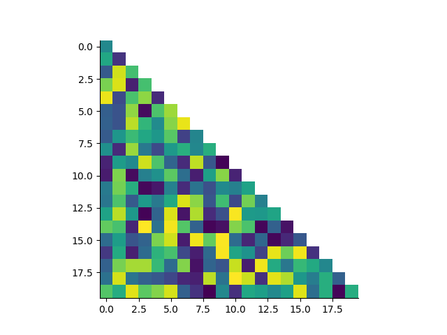
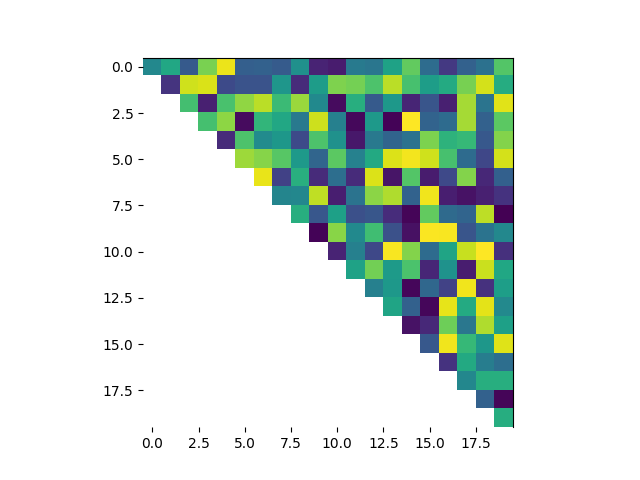
We can decide which portion of heatmap to show using mask argument

x = np.random.random((20, 20))
_ = imshow(x, mask=True)

_ = imshow(x, mask="upper")

_ = imshow(x, mask="lower")

get axes from im and show its processing

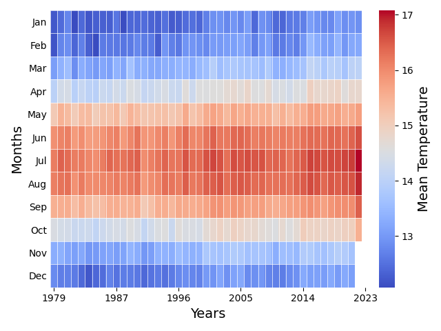
data = pd.read_json('https://climatereanalyzer.org/clim/t2_daily/json_cfsr/cfsr_world_t2_day.json')
index = data.pop('name')
nyrs = 45
data = pd.DataFrame(
    np.array([np.array(data.iloc[row, :].values[0]) for row in range(nyrs)]),
    index=pd.to_datetime(index[0:nyrs])
)
data = data.astype(float)
data1 = pd.concat([data.iloc[i, :] for i in range(data.shape[0])]).dropna()
data1.index = pd.date_range(data.index[0], periods=len(data1), freq="D")
mon_data = data1.resample('ME').mean()

data_np = np.full(shape=(12, nyrs), fill_value=np.nan)
for ii, i in enumerate(range(0, len(mon_data), 12)):
    data_np[:, ii] = mon_data.iloc[i:i + 12].values

print(data_np.shape)

im = imshow(
    data_np,
    cmap="RdBu_r",
    aspect="auto",
    colorbar=True,
    cbar_params=dict(border=False, title="Mean Temperature",
                     title_kws=dict(fontsize=14)),
    show=False,
    ax_kws=dict(xlabel="Years", ylabel="Months",
                xlabel_kws=dict(fontsize=14), ylabel_kws=dict(fontsize=14)),
    grid_params={'border': True, 'color': 'w', 'linewidth': 0.5},
)
im.axes.set_yticks(range(12))
im.axes.set_yticklabels(
    ['Jan','Feb','Mar','Apr','May','Jun','Jul','Aug','Sep','Oct','Nov','Dec'])
im.axes.set_xticks(np.linspace(0, data_np.shape[-1], 6))
im.axes.set_xticklabels(np.linspace(data.index.year.min(), data.index.year.max(), 6, dtype=int))
despine_axes(im.axes)
im.axes.tick_params(axis=u'y', which=u'both',length=0)
ticklabels = []
for ticklabel in im.colorbar.ax.get_yticklabels():
    ticklabel.set_text(f"{ticklabel.get_text()}℃")
    ticklabels.append(ticklabel)
im.colorbar.set_ticklabels(ticklabels)
plt.tight_layout()
plt.show()

(12, 45)
/home/docs/checkouts/readthedocs.org/user_builds/easy-mpl/checkouts/latest/examples/imshow.py:133: UserWarning: set_ticklabels() should only be used with a fixed number of ticks, i.e. after set_ticks() or using a FixedLocator.
  im.colorbar.set_ticklabels(ticklabels)