j. pie

This file shows the usage of pie() function.

import numpy as np
from easy_mpl import pie
import matplotlib.pyplot as plt
import matplotlib.colors as mcolors
from easy_mpl.utils import version_info, map_array_to_cmap

version_info()

# sphinx_gallery_thumbnail_number = 5

{'easy_mpl': '0.21.4', 'matplotlib': '3.8.0', 'numpy': '1.26.1', 'pandas': '2.1.1', 'scipy': '1.11.3'}

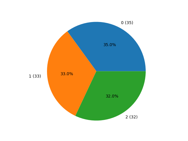
_ = pie(np.random.randint(0, 3, 100))

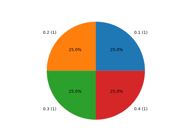
_ = pie([0.2, 0.3, 0.1, 0.4])

# to explode 0.3
explode = (0, 0.1, 0, 0, 0)
_ = pie(fractions=[0.2, 0.3, 0.15, 0.25, 0.1], explode=explode)

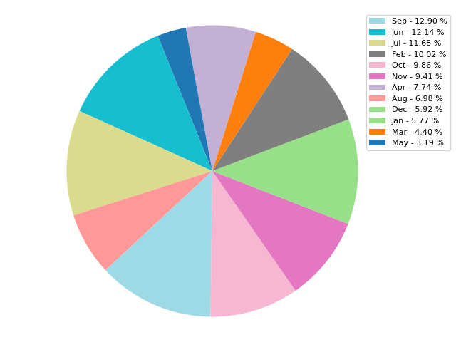
Specifying colors for each section of pie chart

rng = np.random.default_rng(313)
labels = ['Jan','Feb','Mar','Apr','May','Jun','Jul','Aug','Sep','Oct', 'Nov','Dec']
y = rng.integers(10, 100, 12)
colors, _ = map_array_to_cmap(y, cmap="tab20")
percent = 100.*y/y.sum()

outs = pie(fractions=percent, autopct=None,
           colors=colors, show=False)
patches, texts = outs
labels = ['{0} - {1:1.2f} %'.format(i,j) for i,j in zip(labels, percent)]

patches, labels, dummy =  zip(*sorted(zip(patches, labels, y),
                                      key=lambda x: x[2],
                                      reverse=True))

plt.legend(patches, labels, bbox_to_anchor=(1.1, 1.),
           fontsize=8)
plt.tight_layout()
plt.show()

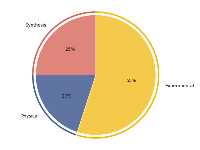
seg_colors = ["#F5B800", "#4461A1", "#DF5F50"]

# Change the saturation of seg_colors to 70% for the interior segments
rgb = mcolors.to_rgba_array(seg_colors)[:,:-1]
hsv = mcolors.rgb_to_hsv(rgb)
hsv[:,1] = 0.7 * hsv[:, 1]
interior_colors = mcolors.hsv_to_rgb(hsv)

pie(fractions=[0.55, 0.2, 0.25],  colors=seg_colors,
       labels=['Experimental', 'Physical', 'Synthesis'],
       wedgeprops=dict(edgecolor="w", width=0.03), radius=1,
autopct=None,
       startangle=90, counterclock=False, show=False)

pie(fractions=[0.55, 0.2, 0.25], colors=interior_colors,
       autopct='%1.0f%%',
       wedgeprops=dict(edgecolor="w"), radius=1-2*0.03,
       startangle=90, counterclock=False, ax=plt.gca(), show=False)

plt.tight_layout()
plt.show()